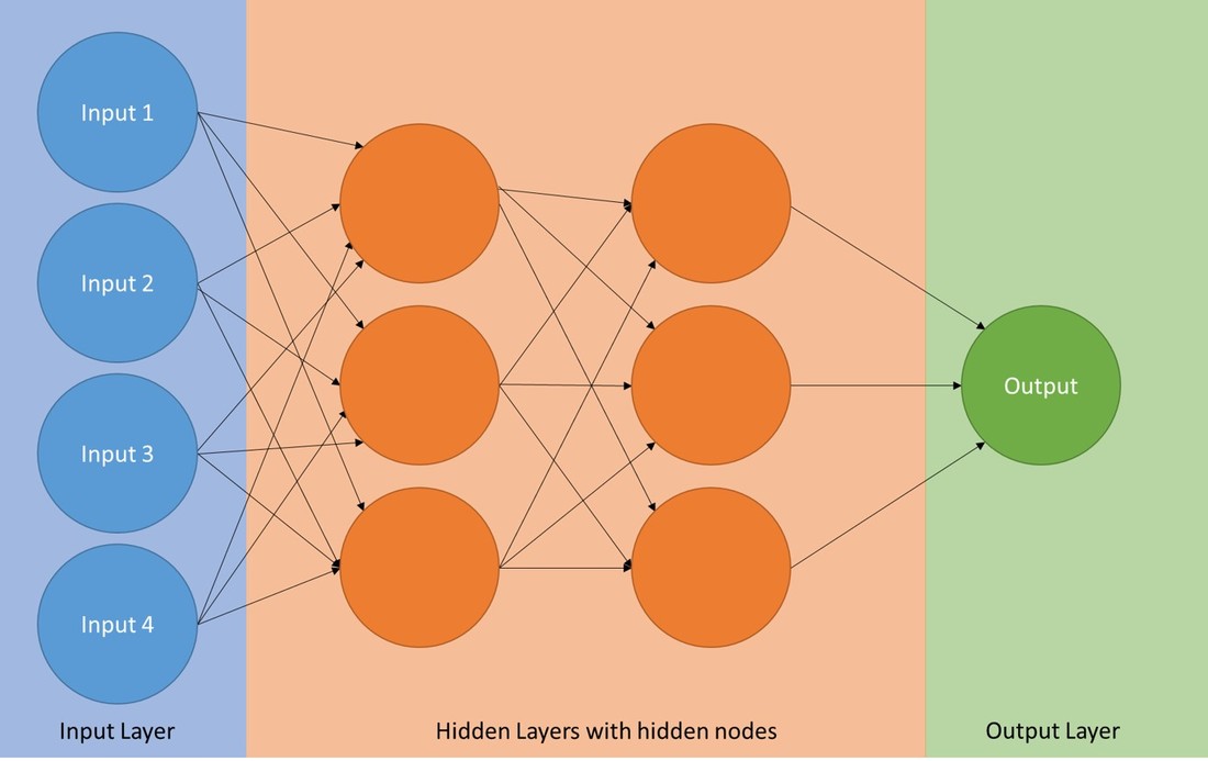
 So-called Artificial Neural Networks (ANN) are a family of popular Machine Learning algorithms that has contributed to advances in data science, e.g. in processing speech, vision and text. In essence, a Neural Network can be seen as a computational system that provides predictions based on existing data. Neural Networks are comparable to non-linear regression models (such as logit regression), their potential strength lies in the ability to process a large number of model parameters. Neural Networks are good at learning non-linear functions. Moreover multiple outputs can be modelled. Artifical Neural Networks are generically inspired by the biological neural networks within animal and human brains. They consist of the following key components:
 For the simplified application example below, we produced an example dataset with some 140.000 records. Imagine that we start with a relatively large dataset of sporadic donors and have come up with a straightforward definition of the dependent churn variable, e.g. a definition based on the recency of the last respective donation. The features (variables) we included were:
We start with loading the relevant R packages, reading in our base dataset and some data pre-processing. Code Snippet #1: Loading packages and data
An essential step in setting up Neural Networks is data normalization. This implies the scaling of the data. See for instance this link for some brief conceptual considerations and information on the scale function in R. Code Snippet #2: Scaling
We then split the dataset into a training and test dataset using a 70% split. Code Snippet #3: Training and test set
Now we are ready to fit the model. We use the package nnet with one hidden layer containing 4 neurons. We run a maximum of 5.000 iterations using the code shown in code snippet number 4: 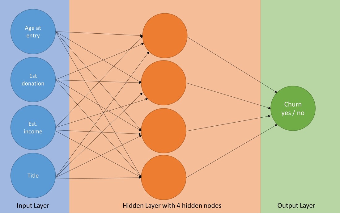 Code Snippet #4: Fitting Neural Net Model
After fitting the model, we plot our neural net object. The neuron B1 in the illustration below is a so called bias unit. This is an additional neuron added to each pre-output layer (in our case one). Bias units are not connected to any previous layer and therefore do not represent an "activity". Bias units can still have outgoing connections and might contribute to the outputs in doing so. There is a compact post on Quora with a more detailed discussion. 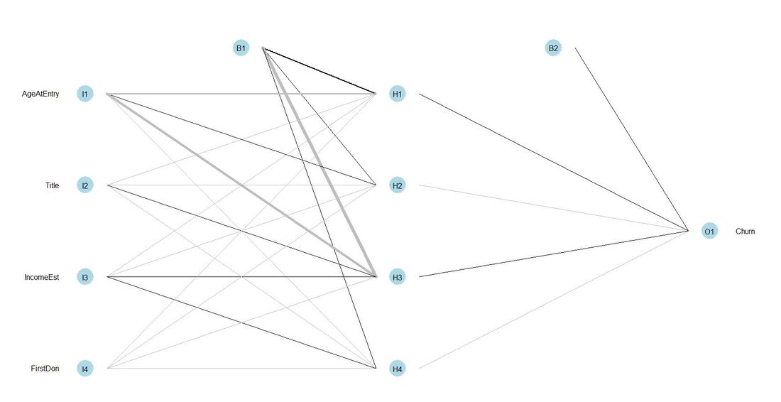 When it comes to modelling in a data science context, it is quite common to look at the variable importance within the respective model. For neural nets, there is a comfortable way to do this using the function olden from the package NeuralNetTools. For our readers interested in the conceptual foundations of this functions, we can recommend this paper. Code Snippet #5: Function olden for variable importance
This is the chart that we get: 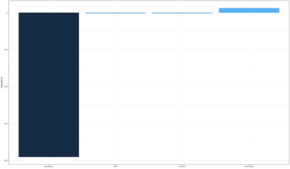 It stand out that the variable Age at entry has a high negative importance on the output whereas Estimated Income shows some degree of positive variable importance. We finally turn to running the neural net model for predictive purposes on our test data set and plot our results in a confusion matrix-like manner: Code Snippet #6: Run prediction and show results
The result of the code above looks as follows: 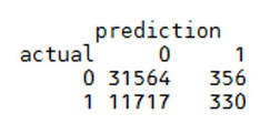 The table above cross-tabls the actual and predicted outcomes of churned and non-churned donors. Let's now evaluate the predictive power of our example neural net. In doing so, we can recommend this nice guide to interpreting confusion matrices which can be found here.
In the light of our data and the example model described above, we can conclude that definitely further model tuning would be needed. Tuning will focus on the used Hyperparameters. At the same time, we would recommend running a "benchmark model" such as a logit regression to compare the neural net's model performance with. As further reading we can recommend:
As always, we look forward to your shares, like, comments and thoughts. Have a nice, hopefully long (rest of) summer!
1 Comment
|