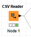
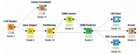
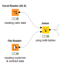
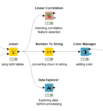
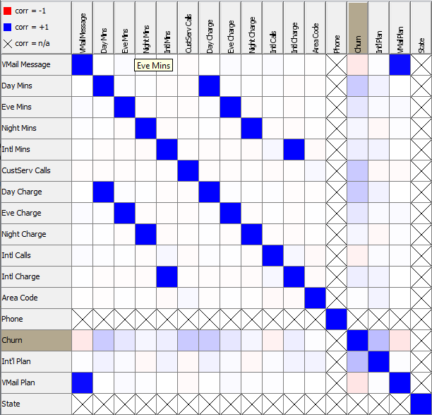
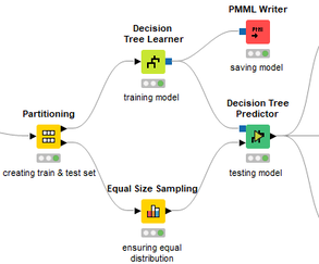
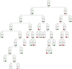
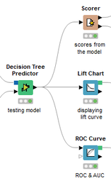
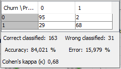
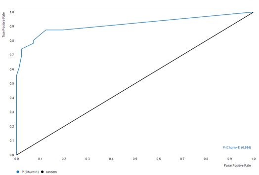
 David Weber, BA Data Science & Analytics “If your only tool is a hammer, then every problem looks like a nail.” – Unknown. Today’s data science landscape is a great example where we need hammers, but we also need screwdrivers, wrenches and pliers. Even though R and Python are the most used programming languages for data science, it is important to expand the toolset with other great utensils. Today’s blog post will introduce a tool, which lets you leverage the benefits of data science without being native in coding: KNIME Analytics Platform. KNIME (Konstanz Information Miner) provides a workflow-based analytics platform that enables you to fully focus on your domain knowledge such as fundraising processes. The intuitive and automatable environment enables guided analytics without knowing how to code. This blog provides you a hands-on demonstration of the key-concepts. Important KNIME TermsBefore we start with a walkthrough of a relevant example, we need to declare some of the most important KNIME terms. Nodes: A node represents a processing point for a certain action. There are many nodes for different tasks, for example reading a CSV-file. You can find further explanations about different nodes on Node Pit. Workflow: A workflow within KNIME is a set of nodes or a sequence of actions you take to accomplish your particular task. Workflows can easily be saved and used by other colleagues. Even collapsing workflows into a single meta-node is possible. That makes them reusable in other workflows. Extensions: KNIME Extensions are an easy and flexible way to extend the platform’s functionalities by providing nodes for certain tasks (connecting to databases, processing data, API requests, etc.). Sample Dataset and Data ImportFor demonstration, we are going to use a telecom dataset for churn prediction. This dataset could be easily replaced with a fundraising dataset containing information about churned donors. Customer or donor churn, also known as customer attrition is a critical metric for every business, especially in the non-profit sector (i.e. quitting regular donations). For more information on donor churn, visit our previous blog posts. Consisting of two tables, the dataset includes call-data from customers and a table about customer contract data. While using some of the information available, we will try to predict whether a customer will quit his subscription or not. Churn is represented with a binary variable (0 = no churn, 1 = churn). For visualization purposes, we are going to use a decision tree classifier, although there are probably even better classification algorithms available. First, we are using an Excel Reader and a File Reader to import both files. To make things easier, we use a Joiner node where we join both tables based on a common key. The result is a single table now ready for exploration and further analysis. Feature EngineeringFeature Engineering is the process of analyzing your data and deciding which parameters have an impact on the label we want to predict – in this case whether a customer will quit or not. In other words: Making your data insightful. But before we look at correlations between the label and the features, a general exploration of our data is recommendable. The Data Explorer node is perfect for some basic information. One thing we notice is that we need to convert our churn label to a string, in order to make it interpretable for our classifier later. This can be done with the Number to String node. Now it’s time for some correlation matrices. We are able to see some correlation between various features and our churn label, whereas others do not correlate really. We decide to get rid of those. Model TrainingNow let’s start with the training of our model. But before we can do that, we need to partition our data into a training- and test-dataset. The training-set (mostly around 60-80% of our data) is used to train our model. The other part of our data will be used to test our model and to make sure it has prediction power. We can verify this with certain metrics. In this case, we will set the partition-percentage to 80%, which seems to be a good amount. This data will be fed into our decision tree learner. After some computing time, our finished decision tree looks like this: In order to make the model reusable and available for predictions with new datasets, we can save it with the PMML Writer node for later use. PMML is a format for sharing and reusing built models. If we want to, we can read the model later on with a PMML Reader node to make predictions with a new, unknown dataset. But before we use our model on a regular basis, we need to evaluate it with our test-dataset, which we split earlier. Model Prediction and EvaluationNow, testing our new model and evaluating its performance is one of the most important steps. If we can’t be sure that our model will predict right to a certain extent, it would be fatal to deploy it. So we feed the Decision Tree Predictor node with our test-dataset. This lets us see how the model performed. We have certain metrics within our KNIME workflow to fully evaluate it. First, we are using a Scorer node to get the confusion matrix and some other important statistics. Our confusion matrix gives us a little hint about threshold tuning, but the accuracy with 84% looks already pretty good. Our model predicted 29 cases as ‘no churn’, although they were actually ‘churning’. This number is rather high, so we should consider tuning our model parameter. Next up is the ROC (Receiver Operating Characteristics) Curve. It maps True Positive Rates and False Positive Rates against each other. One of the results is the AUC (Area under the Curve) which adds up to a very good score of 0.914. A score of 0.5 (the diagonal in the chart below) represents prediction without any meaningfulness, because it means predicting randomly. Additional metrics would be the Lift Chart and Lift Table, but an explanation would be beyond the scope of today’s blog. We think it’s time to summarize and draw a conclusion. Too good to be true?KNIME is a powerful platform, which provides various possibilities to extract, transform, load and analyze your data. However, simplicity has its limitations. In direct comparison with various R packages, visualizations are not as neat and configurable. And the ‘simplistic’ approach to data science limits possibilities in some way or another, requiring the user to have a thorough understanding of the data science pipeline and process. Further, most real life cases are more complicated and need more feature engineering and analysis beforehand – creating the model itself is mostly one of the smallest challenges.
Nevertheless, we think that KNIME is an awesome tool for data engineering / exploration and workflow automation (and building fun stuff with social media and web scraping). But if you are looking for complex models supporting your business decisions – KNIME won’t probably be the platform you are searching for. We hope you liked this month’s blog post and we would love to get in touch if you are interested in achieving advanced insights with your data or just want to dive deeper into the topic. If you want to know what Joint Systems can offer you concerning data analytics, this page will provide you with more information.
2 Comments
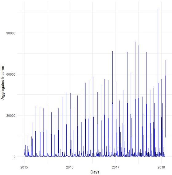
 Every four years, football is omnipresent as national teams compete in the world championship. Like it or not, football is a global obsession on the one hand and big business on the other hand. About a year ago, we first talked about the datafication of football. Data nowadays is used not only used to optimize the performance of players and teams but also to predict the results of football matches and whole tournaments. In our last football related post, we already mentioned Martin Eastwoods presentation from 2014 in which he discussed the application of a Poisson regression model with an adjustment inspired by the 1997 paper by Dixon and Coles published in the Journal of the Royal Statistical Society. Another interesting blog post applying a linear model on Premier league data is from David Sheehan. It is not surprising that many data scientists made an effort to set up prediction models for the coming football world champion that is currently searched for in Russia. Ritchie King, Allison McCann and Matthew Conlen already tried to predict the 2014 world champion (ok, Brazil did not finally make it ...) on fivethirtyeight.com, the site founded by Nate Silver (well known for predicting baseball and election results). Two interesting approaches we found for the current World Cup in Russia use the same data set from kaggle.com containing international football results from 1872 to 2017. While Gerald Muriuki applies a logistic regression model and comes up with Brazil as next world champion, Estefany Torres applies decision trees and predicts Spain to win the tournament. Torres additionally included data on individual player performance and market value in her analysis. James Le took an even closer look at individual player data and investigated the optimal line up for some of the high profile teams in the tournament. We particularly liked the descriptive analyses of the Fifa18 player dataset. Le’s personal prediction is France by the way. We also came across a post on KDnuggets that mentions additional data sources (FIFA world rankings, Elo ratings, TransferMarkt team value and betting odds). The prediction model there – our Northern neighbours might be happy to hear that – sees Germany beating Brazil in the final. We will see on July 15th ... and wish you nice summer days / holidays in the meantime. Read you soon!  Do you sometimes find yourself wishing to predict the future? Well, let's stay down-to-earth, nobody can (not even fundraisers or analysts :-). However, there are established statistical methods in the area of time series that we find potentially interesting in the context of fundraising analytics. Our first blog post of 2018 will take a closer look ... Forecasting with ARIMA It seems that forecasting future sales, website traffic etc. has become quite an imperative in a business context. In methodical terms, time series analyses represent a quite popular approach to generate forecasts. They essentially use historical data to derive predictions for possible future outcomes. We thought it worthwhile to apply a so-called ARIMA (Auto-Regressive Integrated Moving Average) model to fundraising income data from an exemplary fundraising charity. The data used The data for the analysis was taken from a medium-sized example fundraising charity. It comprises income data between January 1st, 2015 and February 7, 2018. We therefore work with some 3 years of income data, coming along as accumulated income sums on the level of booking days. The source of income in our case is from regular givers within a specific fundraising product. We know that the organization has grown both in terms of supporters and derived income in the mentioned segment Preparing the data After having loaded the required R packages, we import our example data it into R, take a look at the first couple of records, format the date accordingly and plot it. It has to be noted that the data was directly extracted from the transactional fundraising system and essentially comes along as "income per booking day". Code Snippet 1: Loading R packages and data + plot
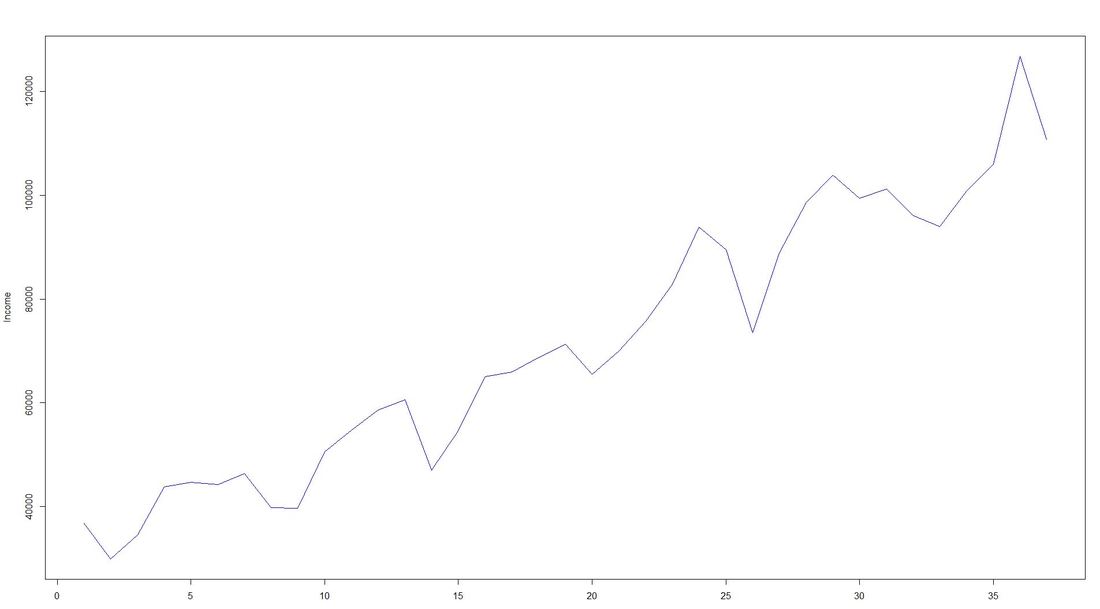
To overcome potential difficulties in modelling at a later stage of the time series analyses, we decided to shorten the date variable and to aggregate on the level of a new date-year-variable. The code and the new plot we generated looks as follows: Code Snippet 2: Date transformation + new plot
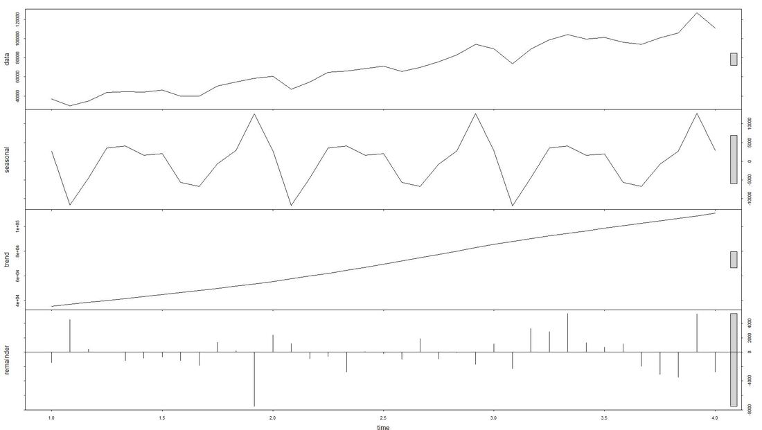
The issue with Stationarity Fitting an ARIMA model requires a time series to be stationary. A stationary time series is one whose properties are independent from the point on the timeline for which its data is observed. From a statistical standpoint, a time series is stationary if its mean, variance, and autocovariance are time-invariant. Time series with underlying trends or seasonality are not stationary. This requirement of stability to apply ARIMA makes intuitive sense: As ARIMA uses previous lags of time series to model its behavior, modeling stable series with consistent properties implies lower uncertainty. The form of the plot from above indicates that the mean is actually not time-invariant - which would violate the stationarity requirement. What to do? We will use the the log of the time-series for the later ARIMA. Decomposing the Data Seasonality, trend, cycle and noise are generic components of a time series. Not every time series will necessarily have all of these components (or even any of them). If they are present, a deconstruction of data can set the baseline for buliding a forecast. The package tseries includes comfortable methods to decompose a time series using stl. It splits the data (which is plotted first using a line chart) into a seasonal component, a trend component and the remainder (i.e. noise). After having transformed that data into a time-series object with ts, we apply stl and plot. Code Snippet 3: Decompose time series + plot
Dealing with Stationarity The augmented Dickey-Fuller (ADF) test is a statistical test for stationarity. The null hypothesis assumes that the series is non-stationary. We now conduct - as mentioned earlier - a log-transformation to the de-seasonalized income and test the data for stationarity using the ADF-test. Code Snippet 4: Apply ADF-Test to logged time series
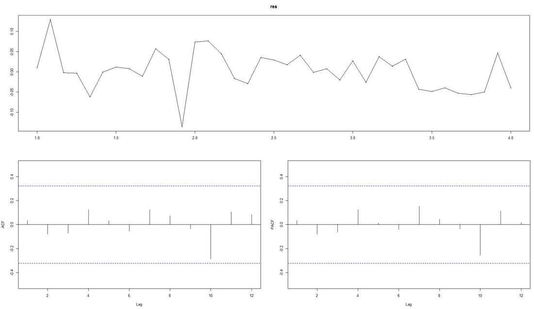
The computed p.value is at 0.0186, i.e the data is stationary and ARIMA can be applied. Fitting the ARIMA Model We now fit the ARIMA model using auto.arima from the package forecast and plot the residuals. Code Snippet 5: Fitting the ARIMA
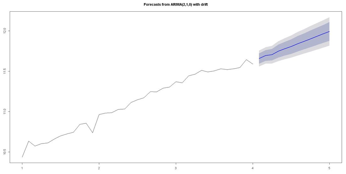
The ACF-plot (Autocorrelation and Cross-Correlation Function Estimation) of the residuals (lower left in picture above) shows that all lags are within the bluish-dotted confidence bands. This implies that the model fit is already quite good and that there are no apparently significant autocorrelations left. The ARIMA model that auto.arima fit was ARIMA(2,1,0) with drift. Forecasting We finally apply the command forecast from the respective package upon the vector fit that contains our ARIMA model. The parameter h represents the number of time series steps to be forcast. In our context this implies predicting the income development for the next 12 months. Code Snippet 6: Forecasting
Outlook and Further reading
We relied on auto.arima which does a lot of tweaking under the hood. There are also ways to modify the ARIMA paramters witin the code. We went through our example with data from regular giver income for which we a priori knew that growth and a certain level of seasonality due to debiting procedures was present. Things might look a little different if we, for instance, worked with campaign-related income or bulk income from a certain channel such as digital. In case you want to take a deeper dive into time series, we recommend the book Time Series Analysis: With Applications in R by Jonathan D. Cryer and Kung-Sik Chan. A free digital textbook called Forecasting: principles and practice by Rob J. Hyndman (author of forecast package) and George Athanasopoulos can also be found on the web. We also found Ruslana Dalinia's blog post on the foundations of time series worth reading. The same goes for the Suresh Kumar Gorakal's introduction of the forecasting package in R. Now it is TIME to say "See you soon" in this SERIES :-)! This month's blog post was contributed by my colleague Susanne Berger. Thank you, Susanne, for the highly interesting read on attrition (churn) for committed givers and how to investigate it with methods and tools from data science. Johannes What this post is about The aim of this post is to gain some insights into the factors driving customer attrition with the aid of a stepwise modeling procedure:
The problem Service-based businesses in the profit as well as in the nonprofit sector are equally confronted with customer attrition (or customer churn). Customer attrition is when customers decide to terminate their commitment (i.e., regular donation), and finds expression in absent interactions and donations. However, any business whose revenue depends on a continued relationship with its customers should focus on this issue. We will try to gain some insights into customer attrition of a selected committed giving product from a fundraising NPO. Acquisition activities for the product took place for six years in total and ended some years ago. Essentially, we are concerned about how long a commitment lasts and what actions can be undertaken to prolong the survival time of commitments. We worked with a pool of some 50.000 observations. To be more specific, we are interested in whether commitments from individuals with a certain sociodemographic profile or other characteristics tend to survive longer. Survival analysis is a tool that helps us to answer these questions. However, it might be the case that the underlying decision process of an individual to terminate a commitment has different influence factors than the decision to start supporting. The approach chosen is to first ask whether an individual with one of the respective commitments has started paying, and if she has, we will have a look at the duration of the commitment. Both of these questions are depicted in a separate model:
The data Let's catch a first glimpse of the data. The variables ComValidFrom and ComValidUntil depict the start- and enddate of a commitment, ComValidDiff gives the length of a commitment in days, and censored shows whether a commitment has a valid enddate and is equal to one if the commitment has been terminated, and equal to zero if the commitment has not been terminated (until 2017-10-14). R Code - Snippet 1
Age and AmountYearly (the yearly amount payable) are, among others variables such as PaymentRhythm, Region and Gender included in the analysis, as they potentially affect the survival time of a commitment or the probability of an individual starting to donate. At the moment, no further explanatory variables are included in the analysis. The analysis After having briefly introduced the most important variables in our data, let's take a look at the results: Has an individual even begun to donate within the committed gift? First, we need to construct a binary variable, that allocates a FALSE if the lifetime sum of a commitment (variable ComLifetimeSum) is zero. Individuals who started to donate if the lifetime sum is larger than zero get assigned a TRUE. The variable DonorStart distinguishes between these two cases. R Code - Snippet 2
A popular way of modeling such binary responses is logistic regression, which is a mathematical model that can be employed to estimate the probability of an individual starting to donate, controlling for certain explanatory variables, as in our case Gender, Age, AmountYearly, PaymentRhythm, and Region. Thus, we fit an exemplary logistic regression model, assuming that Age and AmountYearly have a nonlinear effect on the propability to start paying. In addition, interactions of Age and Gender, as well as of Age and PaymentRhythm are included. For example, the presence of the first interaction effect indicates that the effect of Age on the probability to start to donate is different for male and female individuals. All estimated coeffcients are significant at least at the 5% significance level (except two of the Region coefficients and the main gender effect). R Code - Snippet 3
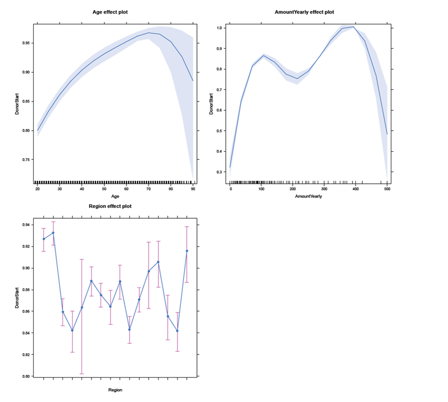
Usually, the results are presented in tables with a lot of information (as for example p-values, standard errors, and test statistics). Furthermore, the estimated coefficients are difficult to translate into an intuitive interpretation, as they are on a log-odds scale. For this reasons, the summary table of the model will not be presented here. An alternative way to show the results is to use some typical values of the explanatory variables to get predicted probabilities of whether an individual started to donate. An effects-plot (from the effects package) plots the results such that we can gain insights into how predicted probabilities change if we vary one explanatory variable while keeping the others constant. R Code - Snippet 4
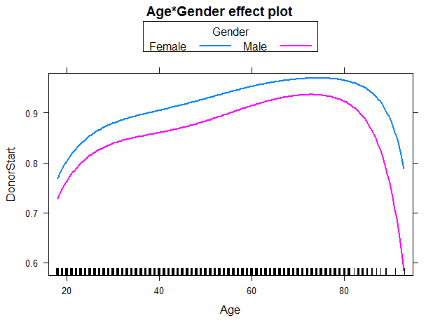
In the subsequent panel, the effects plot for the interaction between Age and Gender is depicted. For all ages, females have a higher probability to start to donate than males. In addition, regardless of gender the older the individual (up to age 70-75), the higher the probability to start to donate. For individuals in their twenties, the steep slope indicates a larger change in probability for each additional year of age than for individuals older than approximately 30 years. We use the following code to create the effects plot: R Code - Snippet 5
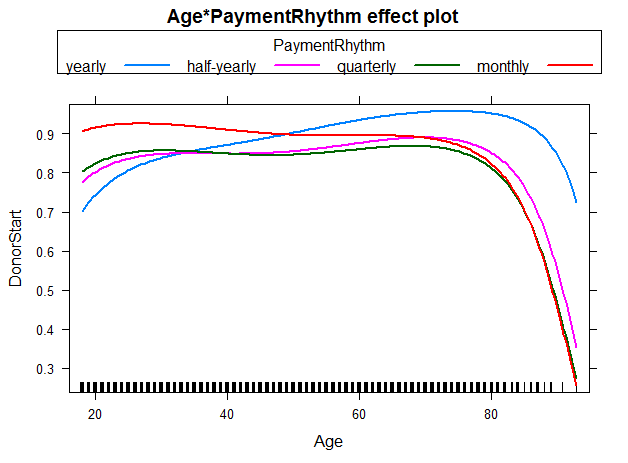
We were also interested in the the interaction between Age and PaymentRhythm. As most of the individuals in the sampe decided for either yearly or half-yearly payment terms, one should not put too much confidence in the other two categories quarterly and monthly. Nevertheless, for individuals with a yearly payment rhythm, the probability to start to donate increases with age up to 70-75 years. For individuals with half-yearly or quarterly payment rhythm, rising age (up to 70-75 years) does not seem to affect the probability of starting to donor much. And for a monthly payment rhythm, the probability even seems to decrease slightly with rising age. The figure below illustrates these findings: R Code - Snippet 6
Now, let's go one step further and try to investigate which factors have an influence on the duration of a commitment, once an individual has started to donate. The question we ask: What affects the duration of a commitment, given the individual acutally started paying for it? Survival analysis analyzes the time to an event, in our case the time until a commitment is terminated. First, we will have a look at a nonparametric Kaplan-Meier estimator, then continue with a semi-parametric Cox proportional hazards (PH) model. For the sake of brevity, we will neither go into the computational details, nor will we discuss model diagnostics and selection. To start the analysis, we first have to load the survival package and create a survival object. R Code - Snippet 7
The variable Survdays reflects the duration of commitments in days. The "+" sign after some observations indicates commitments that are still active (censored), and thus do not have a valid end date (ComValidUntil is set to 2017-10-14 for these cases, as the last valid end date is 2017-10-13): R Code - Snippet 8
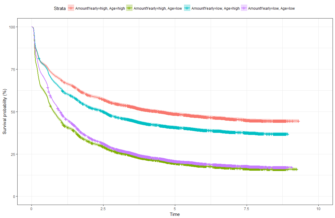
The illustration below shows Kaplan-Meier survival curves for different groups, the tick-marks on the curves represent censored observations. It can be observed that 50% of individuals terminate their commitment approximately within the first 1.5 years. We formed groups using using maximally selected rank statistics: The groups exhibit different survival patterns:
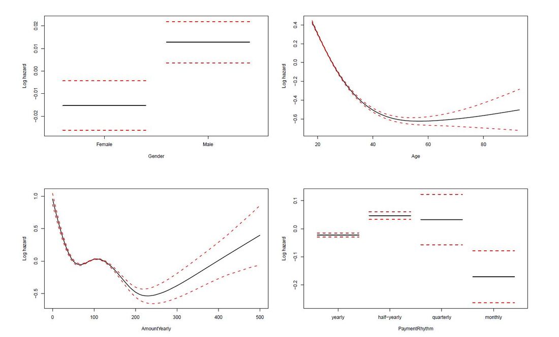
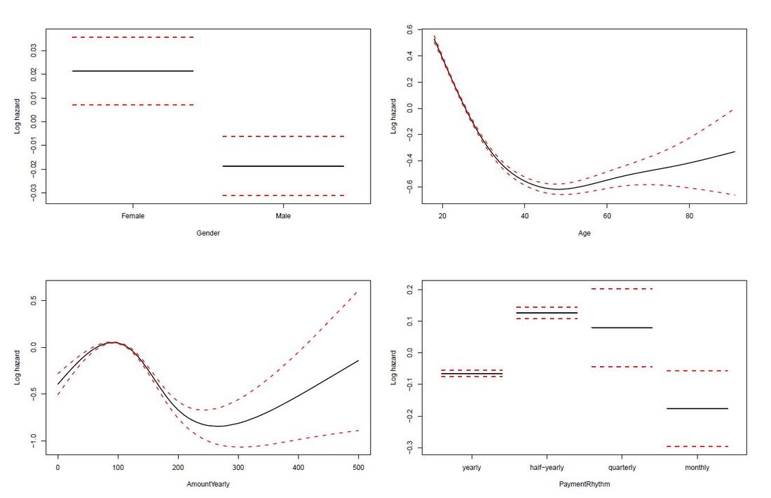
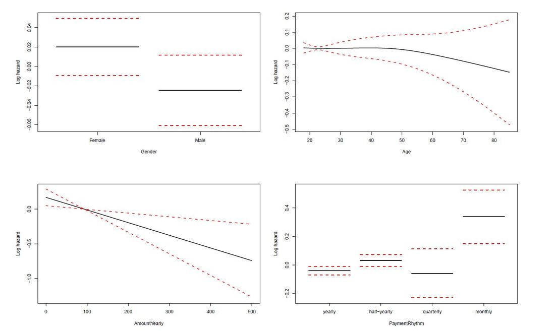
The limit of Kaplan-Meier curves is when several potential variables are available that we believe to contribute to survival. Thus, in a next step we employ a Cox regression model to be able to control statistically for several explanatory variables. Again, we are interested in whether the variables Age, Yearly amount payable, Gender, Payment Rhythm, and Region are related to survival, and if, in what manner. The relationship of Age as well as of Yearly amount payable on the log-hazard (the hazard here is the instantaneous risk - not probability - of attrition) is modelled with a penalized spline in order to account for potential nonlinearities. A Cox proportional hazard model First, we fit one Cox model for all data, including individuals who never started paying their commitments. The upper right panel in the figure below shows that the log hazard decreases (which means a lower relative risk of attrition) with rising age, with a slightly upward turn after age 60. But again, the data are rather sparse at older ages, which is reflected by the wide confidence interval and should thus be interpreted with caution. In the upper left panel, we see that the relative risk of attrition is higher for male than for female individuals. In addition, the lower left Panel depicts a non-linear relationship for the yearly amount payable, the log hazard decreasing the higher the yearly amount, (with a small upward peak at 100 Euro), and increasing again for yearly amounts higher than about 220 Euro (though data are again sparse for amounts higher than 200 Euro). Include only individuals who started to donate... Next, we exclude individuals who never started to donate (i.e. those with a lifetime sum of zero) from the data, and then fit one Cox model for early data (with a commitment duration < 6 months) and one Cox model for later data (with a commitment duration > 6 months). Interestingly, some of the results undergo fundamental changes. ...and a commitment duration of > 6 months In the following, we present the termplots of a Cox model, including only individuals in the analysis who have a commitment duration of more than 6 months, and given the lifetime sum of the commitment is larger than zero. The gender effect turned the other way around compared to the model from the figure above. In addition, the shape of the non-linear effect of the yearly amount payable changed, if only the "later" data are considered. ...and a commitment duration of <= 6 months Last not least the termplots of a further Cox model including only individuals with a commitment duration of less or equal than 6 months, and given the lifetime sum of the commitment is larger than zero are shown. Here, the age effect as well as the yearly amount payable do not seem to exhibit strong nonlinearities (actually, the effect of the yearly amount payable is linear). Furthermore, age does not seem to have an effect on the risk of attrition at all. Conclusion and outlook

The Caret package ("Caret" stands for Classification And REgression Training) includes functions to support the model training process for complex regression and classification problems. It is widely used in the context of Machine Learning which we have dealt with earlier this year. See this blog post from spring if you are interested in an overview. Apart from other, even more advanced algorithms, regression approaches represent and established element of machine learning. There are tons of resources on regression, if you are interested and we will not focus on the basics in this post. There is, however, an earlier post if you look for a brief introduction.
In the following, the output of a knitr report into html was pasted on the blog site. We used made-up data on donor lifetime value as dependent variable and the initial donation, the last donation and donor age as predictors. In short: The explanatory and predictive power of the model are low (for which the dummy data has to be blamed to a certain extent). However, the code you will find below aims to illustrate important concepts of machine learning in R:
Preparing Training and Test DataWe see that InitialDonation, LastDonation and Lifetimesum are factos .. so let´s prepare the data.
As we have a decent dataset now we go ahead and load the promiment machine learning package Caret (Classification And Regression Training) Data cleaningSo called near-zero-variance variables (i.e. variables where the observations are all the same) are cleaned.
IntercorrelationBefore we fit the model, let´s have a look at intercorrelations
Fitting the modelNow it is the moment we fit the (regression) model:
The scatterplot illustrates the relative poorness of the prediction. So: Still some work (data collection, modelling) to be done :-)
The practise-oriented R case study that is mentioned towards the end of this post was also taken from a telecom example. At first glance, coming up with a churn rate is fairly easy and simple maths only. Measure the numbers of distinct customers / donors (or contracts or committed gifts) lost in a defined period (say, a month) and divide it by the number of customers / donors / contracts etc. at the beginning of this period. This is straightforward, simple in its application and can be easily explained – and is therefore a logical first step to tackle churn from an analytical standpoint. An interesting blog post from ecommerce platform provider Shopify offers a discussion on different aspects of churn calculation – and why things are not always as straightforward as they might seem at first glance. With regard to an inferential or predictive approach to churn, the blog KD Nuggets summarizes possible approaches and names two major streams:
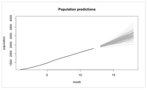
KD Nuggets recommend not to focus too much on one modelling approach but to compare the (particularly predictive) performance of different models. Last, not least they recommend not to forget sound and in-depth explorative analyses as a first step. Will Kurt wrote a highly recommendable, relatively easy to read (caveat: Still take your time to digest it ...) blog post on how to approach churn using a stochastic model of customer population. Have a particular look at the Takeaway and Conclusion part. A summary attempt in one sentence: Although churn is random by its very nature (Brownian motion), suitable modelling will help you (based upon existing data) tell where your customer population will end up in the best and wort case (see picture below - 4.000 customer just will not be reached if we keep on going as we do now ...) Last, not least, if you are interested in a case study from the telecom sector where a Logistic Regression Model was implemented with R, go and have a look at this blog post. The respective R code is also available at Github for the ones interested.
So – enjoy spring if you can and please don´t churn from this blog 😊. |
Categories
All
Archive
June 2024
|
