In modern economy, coming up with forecasts as best possible predictions of future income has become an imperative across industries. Also the charitable nonprofit sector has seen an increasing adaption of forecasting methods in recent years. This is why we already dealt with this topic on this blog some time ago. The endeavour of forecasting is challenging enough in times of economic stability but seems almost impossible after the advent of a „black swans“ like the Corona Virus. Of course, the future is just as uncertain as Ilya Prigogine said. At the same time, there is a familiy of statistical models which not only provides "well-informed" income predictions but particularly help in finding out to what extent current data deviates from the "expected normal". Let us therefore take a closer look at fundraising income forecasting using time series.The basiscs In their book Financial Management for Nonprofit Organizations from 2018 (by the way a recommendable read), Zietlow et al. differentiate between different forecasting types: 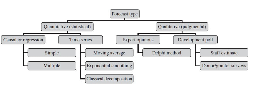 Statistical, forecasting methods can be gernerally divided into causal (also known as regression) methods and time series methods. A causal model is one in which an analyst or data scientist has defined one (simple regression) or several cause factors (multiple regression) for the dependent variable she or he is trying to predict. In the case of income prediction on an aggregated level, drivers (i.e. independent variables) might be found both on the level of donors and exogenous factors. Time series models work differently and tend to be more complex. They essentially use historical data to come up with predictions on future outcomes. Time series are widely used for so called non-stationary data. A stationary time series is one whose properties are independent from the point on the timeline for which its data is observed. From a statistical standpoint, a time series is stationary if its mean, variance, and autocovariance are time-invariant. The requirement of stationarity (i.e. stability) makes intuitive sense as time series use previous lags of time to model developments and modeling stable series with consistent properties implies lower overall uncertainty. Time Series in a Nutshell Time series are often comprised of the following components, although not all time series will necessarily have all or any of them.
The model we will take a closer look at for the prediction of fundraising income is ARIMA which stands for Auto-Regressive Integrated Moving Average. ARIMA models can be seen as the most generic approach to model time series. Wheter the ARIMA algorithm can be applied to the historic income data right away can be evaluated by statistical methods such as the Dickey-Fuller-Test. The null hypothesis of the Dickey-Fuller-Test assumes that the series is non-stationary. Even if this hypothesis cannot be rejected, which means that the data under scrutiny is non-stationary, there are ways to make time series usable. In this case, differencing and log-transformations of the data can be applied in a preparatory step. Applied Example The raw data used for the following example is really straightforward. Historic fundraising income from 2012 to 2019 is extracted in a simple structure (Donor ID, payment date, amount). In a next step, datewise aggregation is applied. Having distinct dates in the dataset allows using both a weekly and monthly perspective on the data. ARIMA is now used to decompose the data. The resulting charts look as follows: 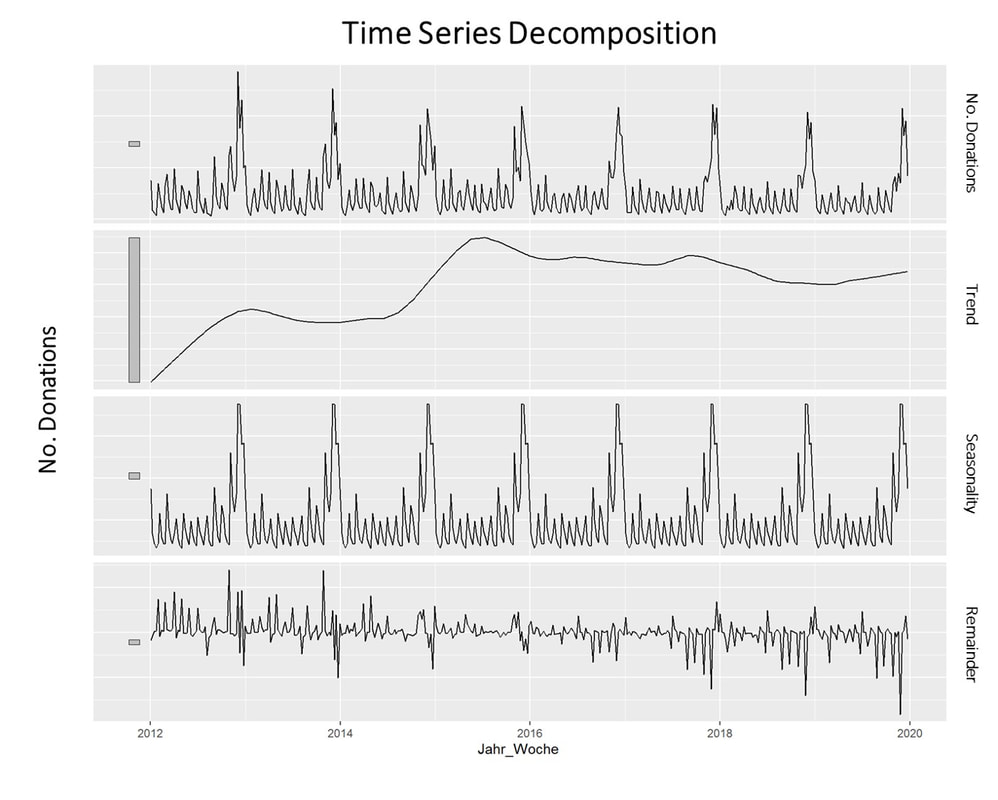 What is clearly visible in the charts above is a degree of seasonality that is obvious in the third box from above but already striking in the overall chart (No. donations, first on top). The second chart from above shows an overall upward trend in the data. For research purposes, we decided to use the data from 2012 to 2018 as "training set" and use ARIMA to generate a prediction for the already closed year 2019. We did that both on the level of accumulated donation counts and donation sum per week. The week-based prediction for the donations looks like this with the blue line being the prediction and the red line being the acutal data: 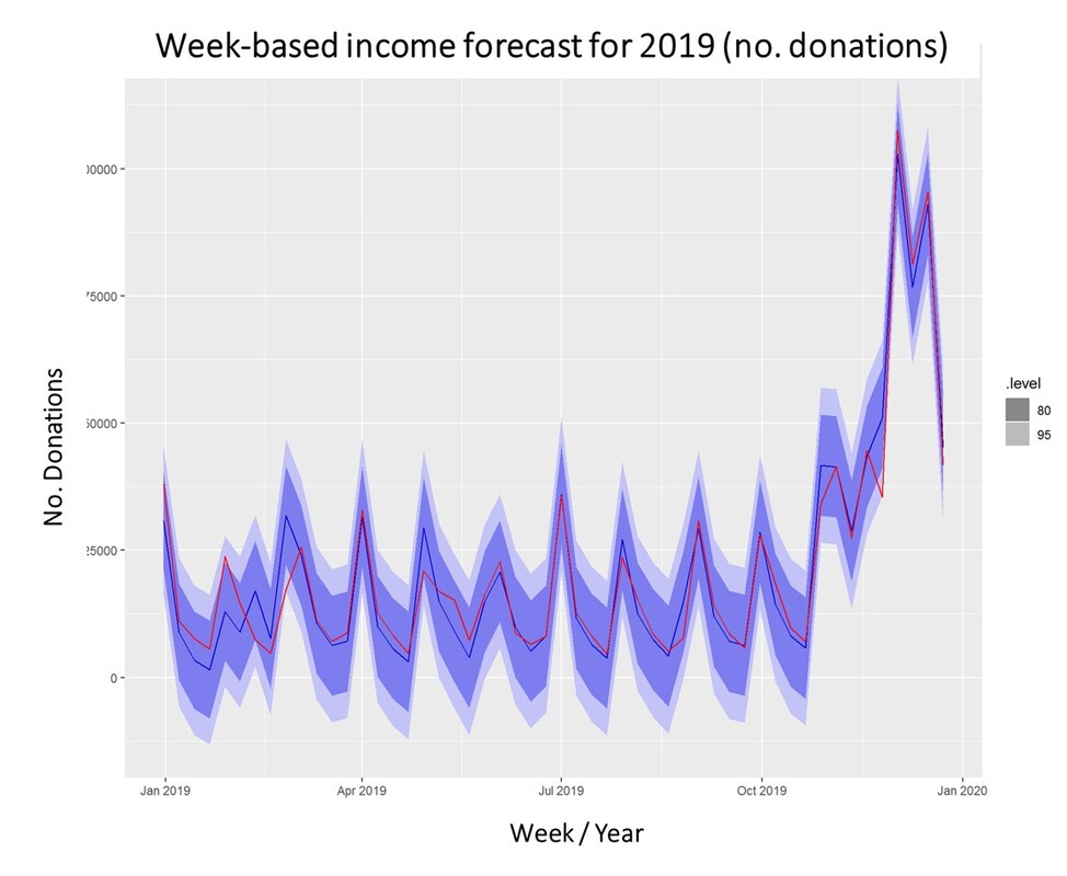 The chart above shows that the blue predicted line generally runs close to the red line representing the actual data. The actual data also oscillates within the forecast prediction intervals at 80% and 95% confidence levels. This is what the actual and predicted data look like for accumulated income over the weeks 2019. 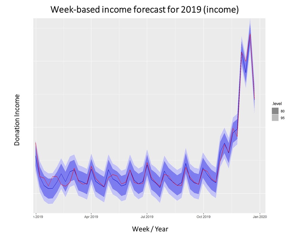 Conclusion To what extent can a time series approach inform fundraising planning and decision making in times of a highly dynamic environment coined by the Corona pandemic? Well, it is still quite unclear how global economy and different countries will develop in the near future. It is also yet to be seen how the Corona crisis will affed fundraising markets on the mid- and long-run. In essence, time series can be an interesting approach to come up with a sophisticated analysis on the extent of the deviation from normal income level, most probably caused by Corona in a direct manner (e.g. face to face fundraising currently stopped) or indirect effects (e.g. rising unemployment) ... We wish you and your dear ones all the best for these challenging times. I think that it is now more than ever worthwhile trying to turn Sophie Scholl´s quote into an attitude: One must have a tough mind - and a soft heart. 
1 Comment
|