by Fabian Pfurtscheller, BSc
Data Science & Analytics at joint systems

More specifically, we will look at correlations between the amount of sporadic donations to a charitable non-profit organization from the period of 2000 to 2019 and three economic data sets from the country the NPO is based in: the national unemployment rate, the national stock market index and an index of economic activity in retail, authored by the national bureau of statistics. We chose these data sets for their ability to paint a picture of the general economic climate, their relatively easy accessibility down to the monthly level and the fact that to the extent that they exhibit seasonality, they do so in the same yearly rhythm as the amount of sporadic donations, simplifying the statistical analyses. The statistical analyses and models employed in this blog post were all implemented in Python, taking heavy use of the statsmodels library.

The main mathematical tool used for the analyses is a time series, which is a set of data points collected over a discrete, ordered time. We have already looked at time series in detail in a past entry on this blog. An important property of time series is that of stationarity, which we discussed here. As in that post, we use the Dickey-Fuller test to investigate whether or not our time series are stationary, which can be done in python like this:

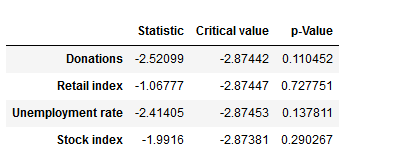
We have defined a function that returns a dataframe with the test statistic, the critical value at a confidence level of 5% and the p-value for the Dickey-Fuller-Test for each time series. The p-values of the test results are above a significance level of 0.05, leading us to keep the null hypothesis of the time series being non-stationary. In cases like these, differencing the time series – this means subtracting the previous value from the current – can help in making the season stationary. However, due to our time series exhibiting strong yearly trends, in our case it makes sense also to take the time series’ seasonal differences, subtracting the values from the year before.

Having prepared our time series, we can look at a first test of interdependencies. Using a version of Pearson’s Chi-Squared test, we examine the (made stationary) series’ Granger causality, which tells us whether data from one series can help in forecasting the future trajectory of another series. The test is applied pairwise on two different time series, with the null hypothesis being that the second time series does not Granger cause the first. The following function returns a data frame that shows the p-values of the tests investigating whether the column variable granger causes the row variable. Especially the first row – indicating (no) Granger causality between the economic data sets on the one hand and the amount of sporadic donations on the other – is interesting to us. At a significance level of 0.05, we keep the null hypothesis of no Granger causality between the economic indicators and the sporadic donations for all three time series.

A second useful quality to look at is cointegration.  We consider a set of time series cointegrated if there exists a linear combination of the time series that is stationary. Cointegrated time series share a common, long-term equilibrium and we can use them to predict each other’s future trajectory using a process called Vector autoregression (VAR). A common test for cointegration is the Johansen cointegration test. In the following, we define a function that returns a dataframe with the test statistic and the critical values of the Johansen test, leading to these results:

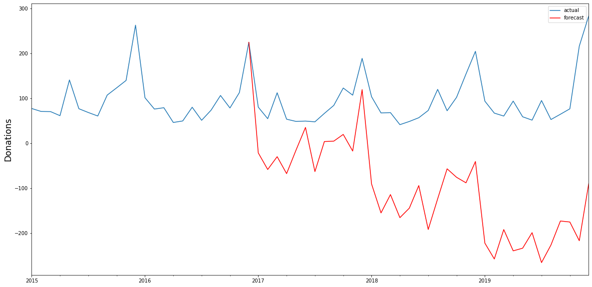
The test statistic is below the critical value for all four of our time series, meaning that we have to keep the null hypothesis of no cointegration and cannot assume the time series to be cointegrated. We can thus not assume that there is an underlying equilibrium between the four time series, and the test results do not support the hypothesis that we can use the time series to forecast each other’s future trajectory.

Had the test results been different and had we been able to reject our null hypothesis, we could have attempted to construct a VAR-model. If we ignore our test results for a moment and do so anyway, we can immediately see that the model falls catastrophically short. The black line in the below graphs show the actual time series of sporadic donations. Having used data until 2016 as our training set, we constructed with the Python library statsmodels a VAR-model that we can use to forecast the sporadic donations from 2017 to 2019 – the red line in the graph – using the actual data for these years for evaluation. As we can see, the model is not able to forecast the amount of sporadic donations very well, capturing the seasonality, but failing to accurately predict the trend and overall trajectory.

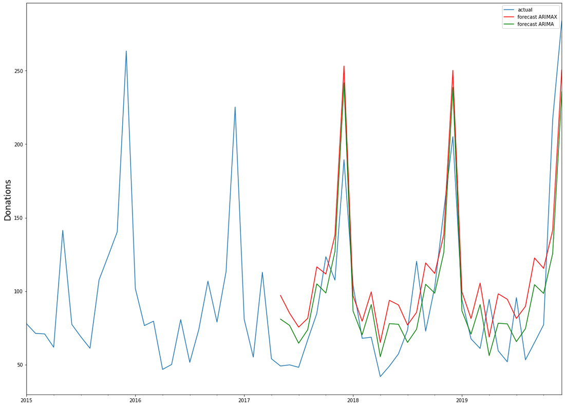
Using a different model does not yield any much better results. We attempted to construct an ARIMAX-model, a generalisation of the ARIMA-model, which we have used previously in this blog, that also takes into account data from external variables – in our case, the economic time series. ARIMA models are composed of three parts: AR for autoregression, indicating a regression on the time series’ past values, I for integration, signifying differencing terms in the case of a non-stationary time series, and MA for the moving-average-model, a regression on past values white noise terms. ARIMAX takes all three of those terms and adds data from external variables – a different time series – to better forecast the time series at hand. Both ARIMA and ARIMAX are implemented in python as part of the statsmodels library, while the pmdarima library comes with an autoarima function modelled on R’s autoarima function, allowing for a quick search through the possible parameters of the ARIMA(X) model.

We have used all four time series to construct an ARIMAX-model, using the economic data to help forecast the amount of sporadic donations. Again we used the data until 2016 as our training set, with the data from 2017 to 2020 as a test set to evaluate results. We have also used a standard ARIMA-model to construct a forecast for sporadic donations only on the time series’ historical data. Interestingly, the models’ projected forecasts did not differ much from each other:

It seems thus that the economic data we have provided – the unemployment rate, the stock index and a retail index – did not add much extra information to better forecast the amount of sporadic donations. Upon closer inspection the ARIMA-model, relying solely on historical data from the time series itself, even performed slightly better. In light of the previous test results – the lack of Granger causality and cointegration – this points to the fact that those economic indicators have little measurable effect on the development of sporadic donations, and thus cannot be used to improve forecasting models for the amount of sporadic donations in the future. However, we believe that the approach of using time series analysis for fundraising income predictions hand in hand with open (economic) data deserves further focus as other base data, time frames, data sources etc. 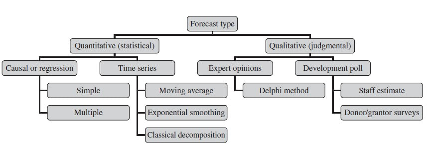might lead to different results!

​The basiscs
​
In their book Financial Management for Nonprofit Organizations from 2018 (by the way a recommendable read), Zietlow et al. differentiate between different forecasting types:

Statistical, forecasting methods can be gernerally divided into causal (also known as regression) methods and time series methods. A causal model is one in which an analyst or data scientist has defined one (simple regression) or several cause factors (multiple regression) for the dependent variable she or he is trying to predict. In the case of income prediction on an aggregated level, drivers (i.e. independent variables) might be found both on the level of donors and exogenous factors. 

Time series models work differently and tend to be more complex. They essentially use historical data to come up with predictions on future outcomes. Time series are widely used for so called non-stationary data. A stationary time series is one whose properties are independent from the point on the timeline for which its data is observed. From a statistical standpoint, a time series is stationary if its mean, variance, and autocovariance are time-invariant. The requirement of stationarity (i.e. stability) makes intuitive sense as time series use previous lags of time to model developments and modeling stable series with consistent properties implies lower overall uncertainty.

Time Series in a Nutshell
​
Time series are often comprised of the following components, although not all time series will necessarily have all or any of them.

• Trend: The time series contains a trend when there is a long-term increase or decrease in the data. This trend does not have to be linear.
• Seasonal: A seasonal pattern exists when a time series is affected by seasonal factors such as month(s) of a year or certain weekdays.
• Cycle: A cylce is there when the data shows rises and falls that are not fixed in frequencies. The respective fluctuations are often related to economic conditions.
• Noise: Remaining random variation in the data.

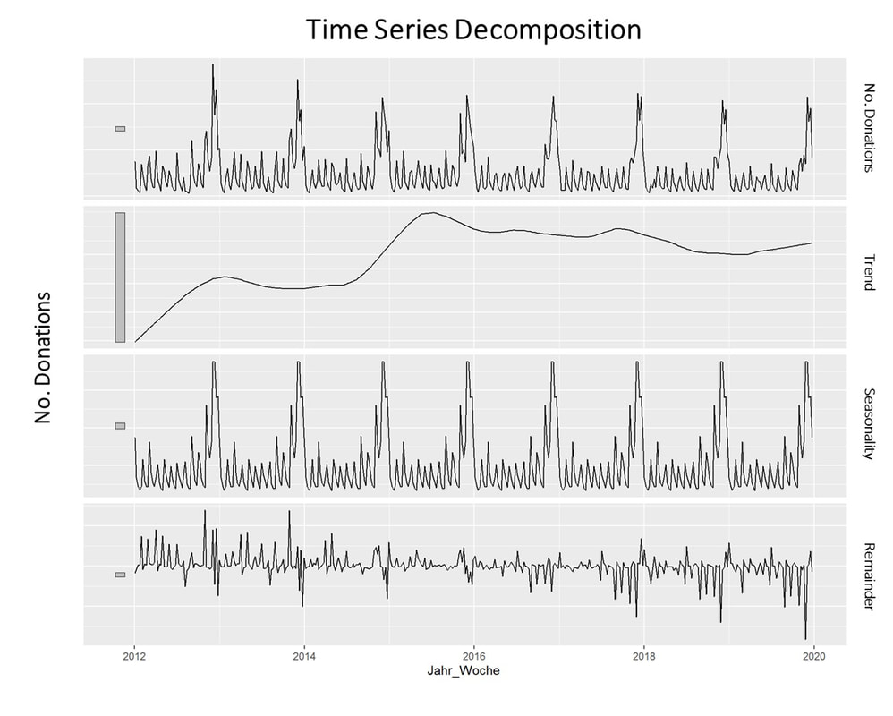
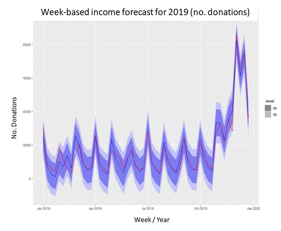
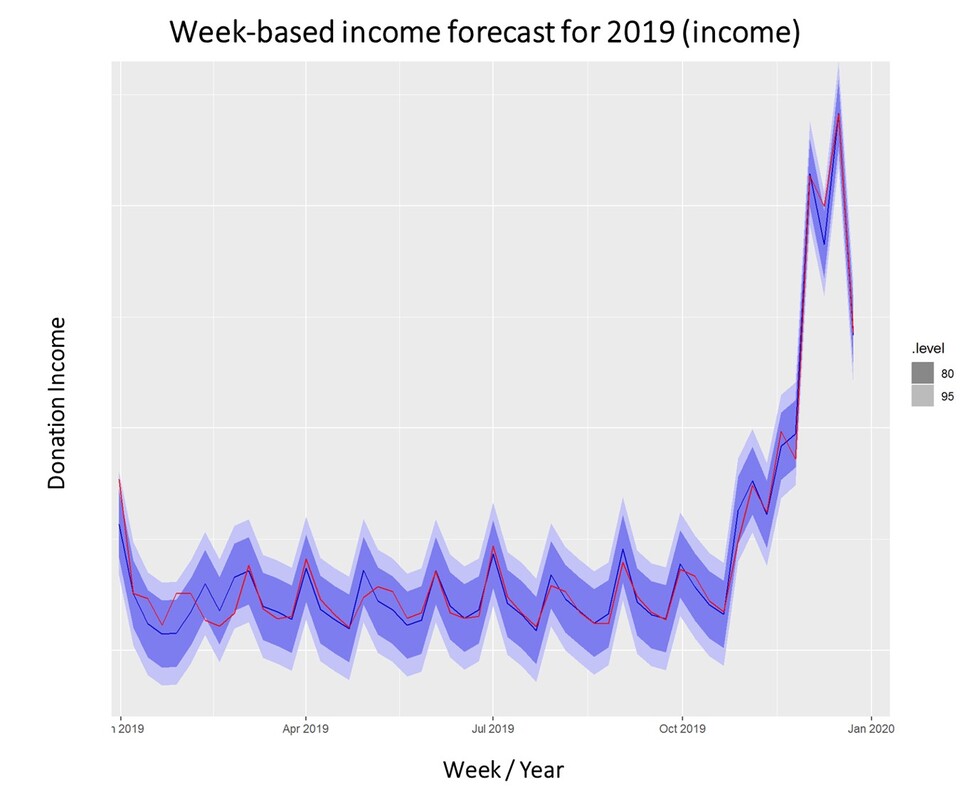
The model we will take a closer look at for the prediction of fundraising income is ARIMA which stands for Auto-Regressive Integrated Moving Average. ARIMA models can be seen as the most generic approach to model time series. Wheter the ARIMA algorithm can be applied to the historic income data right away can be evaluated by statistical methods such as the Dickey-Fuller-Test. The null hypothesis of the Dickey-Fuller-Test assumes that the series is non-stationary. Even if this hypothesis cannot be rejected, which means that the data under scrutiny is non-stationary, there are ways to make time series usable. In this case, differencing and log-transformations of the data can be applied in a preparatory step.

Applied Example

The raw data used for the following example is really straightforward. Historic fundraising income from 2012 to 2019 is extracted in a simple structure (Donor ID, payment date, amount). In a next step, datewise aggregation is applied. Having distinct dates in the dataset allows using both a weekly and monthly perspective on the data. ARIMA is now used to decompose the data. The resulting charts look as follows:
​​

What is clearly visible in the charts above is a degree of seasonality that is obvious in the third box from above but already striking in the overall chart (No. donations, first on top). The second chart from above shows an overall upward trend in the data.
​
​For research purposes, we decided to use the data from 2012 to 2018 as "training set" and use ARIMA to generate a prediction for the already closed year 2019. We did that both on the level of  accumulated donation counts and donation sum per week. The week-based prediction for the donations looks like this with the ​blue line being the prediction and the ​red line being the ​acutal data:
​

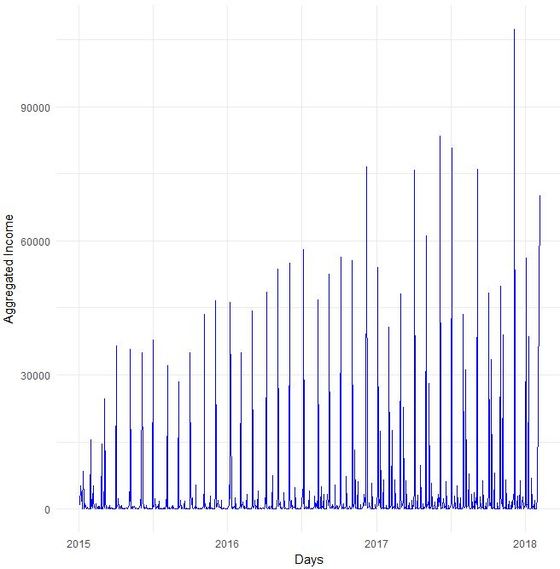
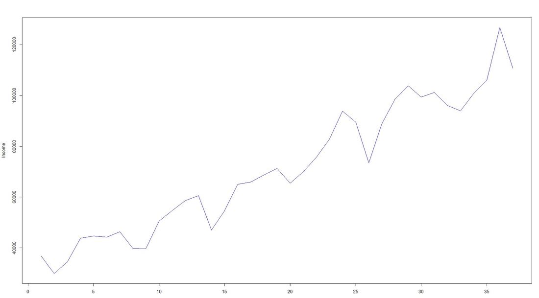
Forecasting with ARIMA

It seems that forecasting future sales, website traffic etc. has become quite an imperative in a business context. In methodical terms, time series analyses represent a quite popular approach to generate forecasts. They essentially use historical data to derive predictions for possible future outcomes. We thought it worthwhile to apply a so-called ARIMA (Auto-Regressive Integrated Moving Average) model to fundraising income data from an exemplary fundraising charity. 

The data used

The data for the analysis was taken from a medium-sized example fundraising charity. It comprises income data between January 1st, 2015 and February 7, 2018. We therefore work with some 3 years of income data, coming along as accumulated income sums on the level of booking days. The source of income in our case is from regular givers within a specific fundraising product. We know that the organization has grown both in terms of supporters and derived income in the mentioned segment

Preparing the data

After having loaded the required R packages, we import our example data it into R, take a look at the first couple of records, format the date accordingly and plot it. It has to be noted that the data  was directly extracted from the transactional fundraising system and essentially comes along as "income per booking day".

To overcome potential difficulties in modelling at a later stage of the time series analyses, we decided to shorten the date variable and to aggregate on the level of a new date-year-variable. The code and the new plot we generated looks as follows:

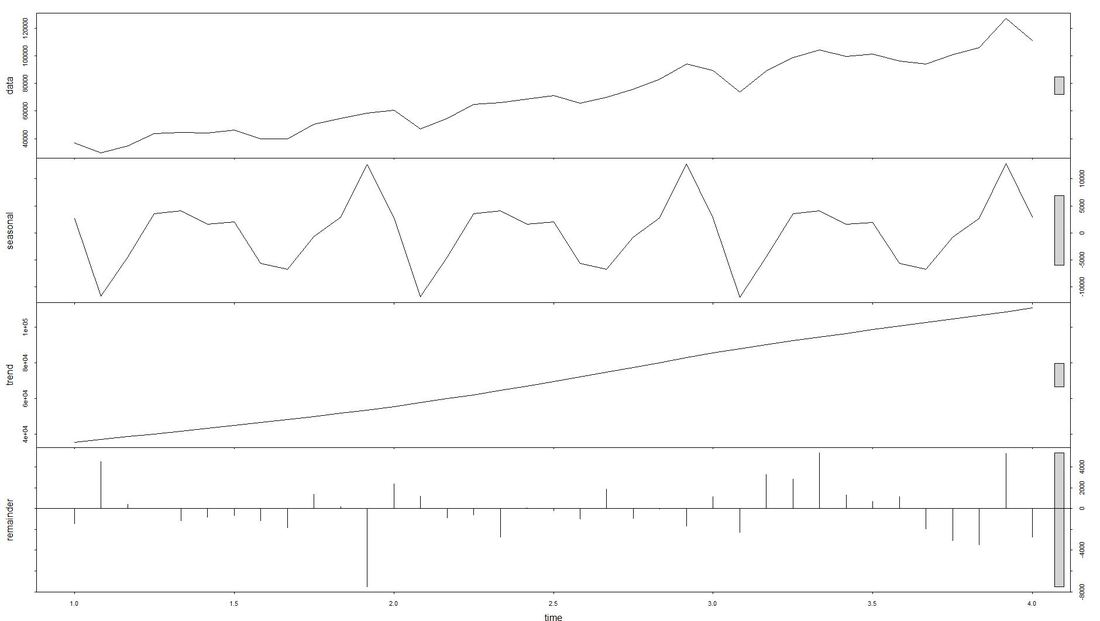
The issue with Stationarity

Fitting an ARIMA model requires a time series to be stationary. A stationary time series is one whose properties are independent from the point on the timeline for which its data is observed. From a statistical standpoint, a time series is stationary if its mean, variance, and autocovariance are time-invariant.

Time series with underlying trends or seasonality are not stationary. This requirement of stability to apply ARIMA makes intuitive sense: As ARIMA uses previous lags of time series to model its behavior, modeling stable series with consistent properties implies lower uncertainty.

The form of the plot from above indicates that the mean is actually not time-invariant - which would violate the stationarity requirement. What to do? We will use the the log of the time-series for the later ARIMA.

Decomposing the Data

Seasonality, trend, cycle and noise are generic components of a time series. Not every time series will necessarily have all of these components (or even any of them). If they are present, a deconstruction of data can set the baseline for buliding a forecast.

The package tseries includes comfortable methods to decompose a time series using stl. It splits the data (which is plotted first using a line chart) into a seasonal component, a trend component and the remainder (i.e. noise). After having transformed that data into a time-series object with ts, we apply stl and plot.

Dealing with Stationarity

The augmented Dickey-Fuller (ADF) test is a statistical test for stationarity. The null hypothesis assumes that the series is non-stationary.

We now conduct - as mentioned earlier - a log-transformation to the de-seasonalized income and test the data for stationarity using the ADF-test.

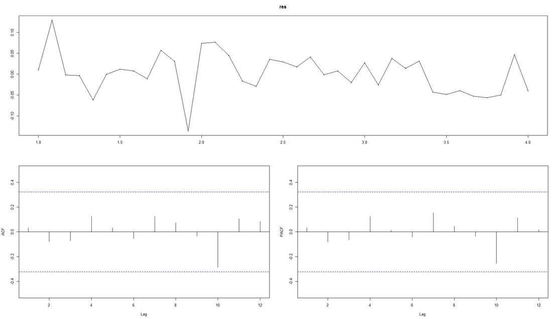
The computed p.value is at 0.0186, i.e the data is stationary and ARIMA can be applied.

Fitting the ARIMA Model

We now fit the ARIMA model using auto.arima from the package forecast and plot the residuals.

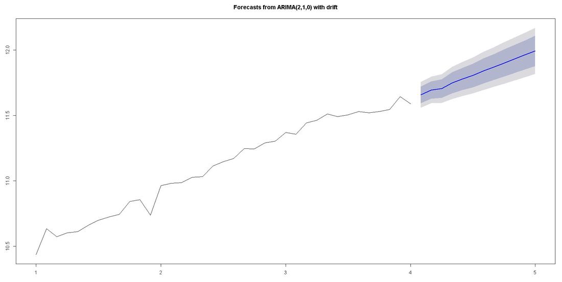
The ACF-plot (Autocorrelation and Cross-Correlation Function Estimation) of the residuals (lower left in picture above) shows that all lags are within the bluish-dotted confidence bands. This implies that the model fit is already quite good and that there are no apparently significant autocorrelations left. The ARIMA  model that auto.arima fit was ARIMA(2,1,0) with drift.

Forecasting

We finally apply the command forecast from the respective package upon the vector fit that contains our ARIMA model. The parameter h represents the number of time series steps to be forcast. In our context this implies predicting the income development for the next 12 months.