|
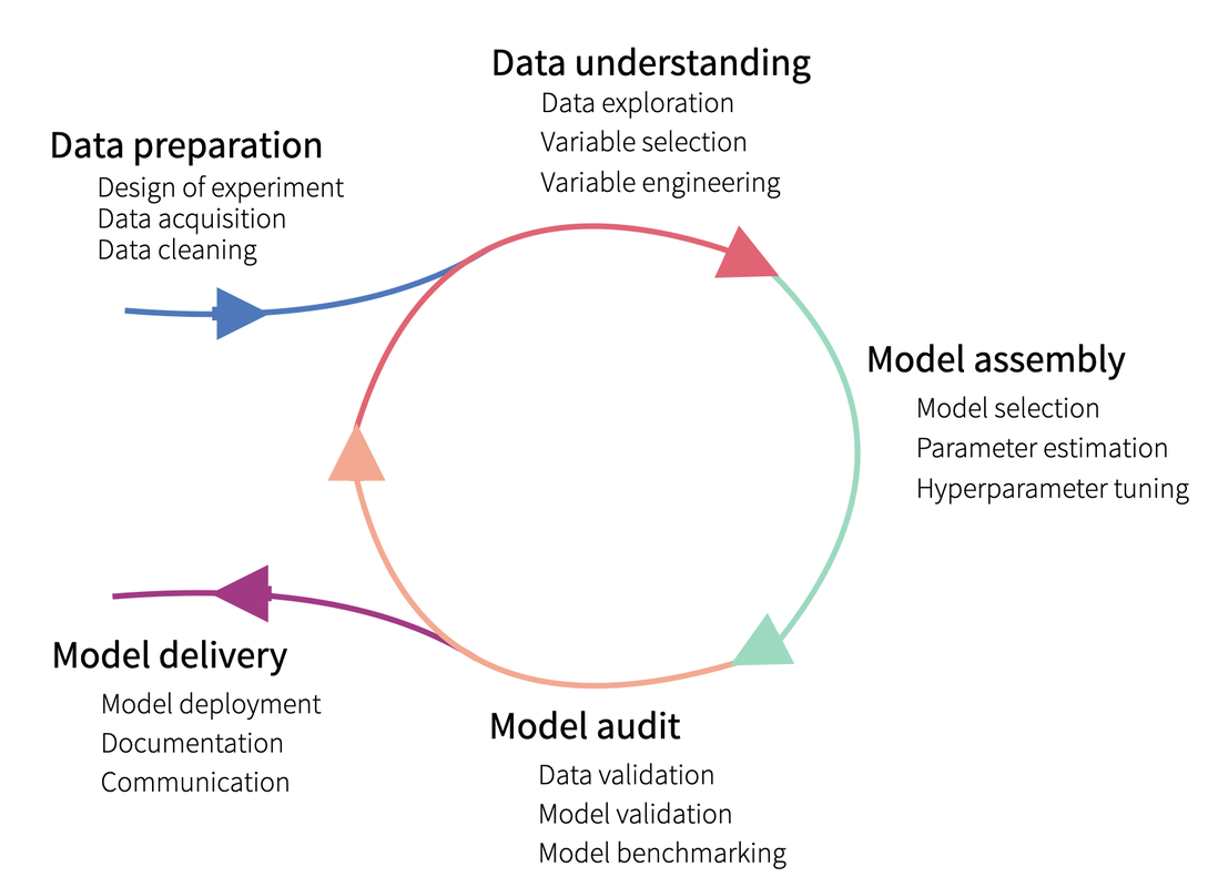
For the last decades, lots of efforts have been put in developing machine learning algorithms and methods. Those methods are currently being widely used among companies and let us extract meaningful insights from our raw data to solve complex problems that could hardly be solved otherwise. They make our life (and our job) easier, but at what cost? There is a good reason why Machine learning methods are known as being “black-box”: They have turned so complex that is hard to know what is exactly going on inside them. However, understanding how models work and making sure our predictions make any sense is an important issue in any business environment. We need to trust our model and our predictions in order to apply them for business decisions. Understanding the model also help us debug it, potentially detect bias, data leakage and wrong behaviour. Towards interpretability: The importance of knowing our data We should take into account that, whenever we talk about modelling, there needs to be a lot of work behind related to data preparation and understanding. Starting with the clients’ needs or interest, those need to be translated into a proper business question, upon which we will then design an experiment. That design should specify, not just the desired output and the proper model to use for it, but also – and more important – the data needed for it. That data needs to exist, be queried and have enough quality to be used. Of course, data also needs to be explored and useful variables (i.e. variables related to the output of interest) be selected. In other words: Modelling is not an isolated process and its results cannot be understood without first understanding the data that has been used to get those results, as well as its relationship with the predicted outcome. Interpretable vs. non interpretable models Until now, we have just talked about black-box models. But are actually all models hard to interpret? The answer is no. Some models are simpler and intrinsically interpretable, including linear models and decision trees. But since that decrease in complexity comes with a cost on the performance, we usually tend to use more complex models, which are hardly interpretable. Or are they? Actually, intensive research has been put into developing model interpretability methods and two main type of methods exist:
Those model methods can also be grouped, depending on their predictions scope, into:
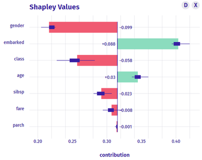
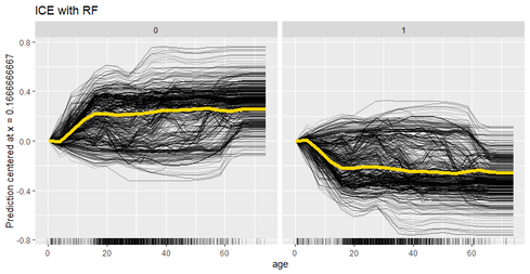
Some Global interpretability examples As previously mentioned, probably the most widely method used is the calculation of the feature importance, and many packages have their own functions to calculate it. For instance, package caret has the function varImp(), which we have used to plot the following example. There, we can see how feature “gender-male” and “age” seem to be the most important features to predict the survival probability in the titanic (yes! we have used the famous Kaggle titanic-dataset to build our models). 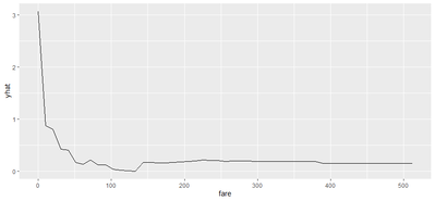 Partial dependence plots are also widely used. These plots show how predicted output changes when we change the values on a given predictor variable. In other words, it shows the effect of single features on the predicted outcome, controlling for the values of all other features. In order to build them, function partial() from package pdp can be used. For instance, in the following partial depende plot we can see how paying a low fare seems to have a positive effect on the survival – which makes sense, knowing for instance that children had preference on the boats! Some local interpretability examples Local interpretability techniques can be studied with the packages DALEX and modelStudio, which let us use a very nice and interactive dashboard – where we can choose which methods and which observations are we most interested at. 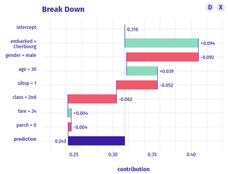 One of the best methods contained are the so-called break-down plots, which show how the contributions attributed to individual explanatory variables change the mean model prediction to yield the actual prediction for a particular single observation. In the following example of a 30 year old male travelling on 2nd class, which payed 24 pounds and boarded in Cherbourg, we can see how the boarding port and the age had a positive contribution on the survival prediction, whereas his gender and the class had a negative one. In this way, we can study each of the observations which we want or have to focus on – for instance, if we think that the model is not working properly on them. Shap values is a similar method, which consists on taking each feature and testing the accuracy of every combination of the rest of features, checking then how adding that feature on each combination improves the accuracy of the prediction. On the following example, and for the same observation as we just analysed, we can see that result are very similar: gender shows the biggest and most negative contribution, while the boarding port has the biggest and most positive effect on the survival prediction, for that specific passenger. Last, if we are interested on how observations’ predictions change when changing feature values, we can study the individual conditional expectation plots. Even though they can just display one feature at a time, it let us have a feeling on how predictions change when feature values change. For instance, on the following example we can see how increasing the age have a negative effect on the survival of the titanic passengers. Some last words
In this post, we have made a brief introduction on the interpretability of machine learning models, we have explained why is important to actually be able to interpret our results and we have shown some of the most used methods. But just as a reminder: for a similar performance, we should actually always prefer simpler models which are interpretable per se, over super complex machine learning ones!
0 Comments
|
Categories
All
Archive
June 2024
|

