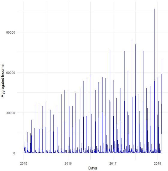
 Do you sometimes find yourself wishing to predict the future? Well, let's stay down-to-earth, nobody can (not even fundraisers or analysts :-). However, there are established statistical methods in the area of time series that we find potentially interesting in the context of fundraising analytics. Our first blog post of 2018 will take a closer look ... Forecasting with ARIMA It seems that forecasting future sales, website traffic etc. has become quite an imperative in a business context. In methodical terms, time series analyses represent a quite popular approach to generate forecasts. They essentially use historical data to derive predictions for possible future outcomes. We thought it worthwhile to apply a so-called ARIMA (Auto-Regressive Integrated Moving Average) model to fundraising income data from an exemplary fundraising charity. The data used The data for the analysis was taken from a medium-sized example fundraising charity. It comprises income data between January 1st, 2015 and February 7, 2018. We therefore work with some 3 years of income data, coming along as accumulated income sums on the level of booking days. The source of income in our case is from regular givers within a specific fundraising product. We know that the organization has grown both in terms of supporters and derived income in the mentioned segment Preparing the data After having loaded the required R packages, we import our example data it into R, take a look at the first couple of records, format the date accordingly and plot it. It has to be noted that the data was directly extracted from the transactional fundraising system and essentially comes along as "income per booking day". Code Snippet 1: Loading R packages and data + plot
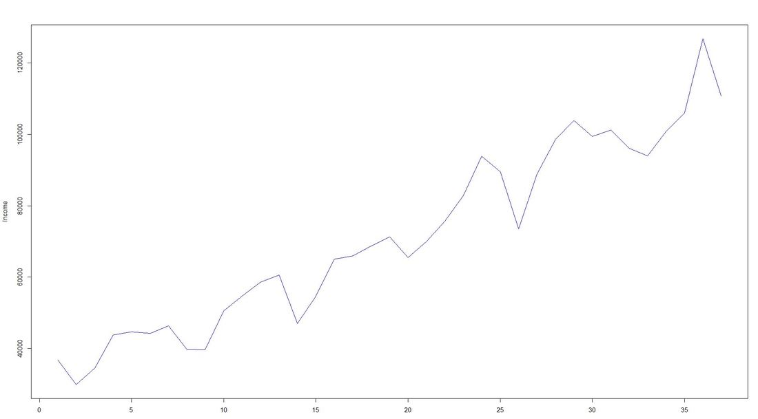
 To overcome potential difficulties in modelling at a later stage of the time series analyses, we decided to shorten the date variable and to aggregate on the level of a new date-year-variable. The code and the new plot we generated looks as follows: Code Snippet 2: Date transformation + new plot
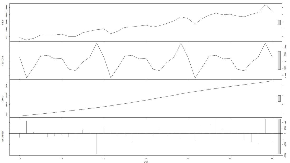
 The issue with Stationarity Fitting an ARIMA model requires a time series to be stationary. A stationary time series is one whose properties are independent from the point on the timeline for which its data is observed. From a statistical standpoint, a time series is stationary if its mean, variance, and autocovariance are time-invariant. Time series with underlying trends or seasonality are not stationary. This requirement of stability to apply ARIMA makes intuitive sense: As ARIMA uses previous lags of time series to model its behavior, modeling stable series with consistent properties implies lower uncertainty. The form of the plot from above indicates that the mean is actually not time-invariant - which would violate the stationarity requirement. What to do? We will use the the log of the time-series for the later ARIMA. Decomposing the Data Seasonality, trend, cycle and noise are generic components of a time series. Not every time series will necessarily have all of these components (or even any of them). If they are present, a deconstruction of data can set the baseline for buliding a forecast. The package tseries includes comfortable methods to decompose a time series using stl. It splits the data (which is plotted first using a line chart) into a seasonal component, a trend component and the remainder (i.e. noise). After having transformed that data into a time-series object with ts, we apply stl and plot. Code Snippet 3: Decompose time series + plot
 Dealing with Stationarity The augmented Dickey-Fuller (ADF) test is a statistical test for stationarity. The null hypothesis assumes that the series is non-stationary. We now conduct - as mentioned earlier - a log-transformation to the de-seasonalized income and test the data for stationarity using the ADF-test. Code Snippet 4: Apply ADF-Test to logged time series
The computed p.value is at 0.0186, i.e the data is stationary and ARIMA can be applied. Fitting the ARIMA Model We now fit the ARIMA model using auto.arima from the package forecast and plot the residuals. Code Snippet 5: Fitting the ARIMA
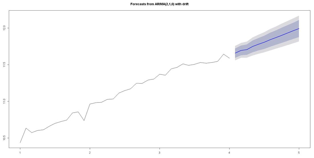
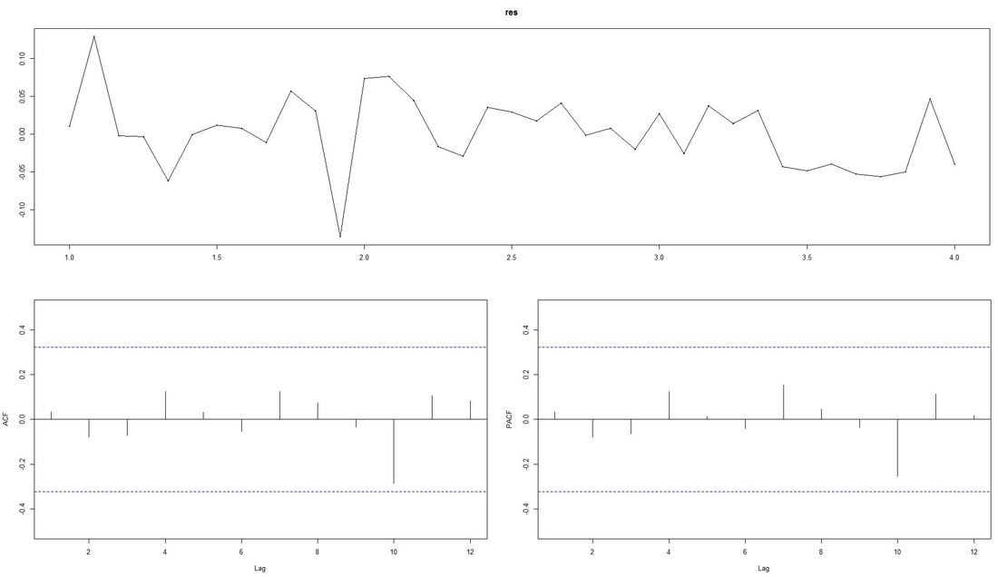 The ACF-plot (Autocorrelation and Cross-Correlation Function Estimation) of the residuals (lower left in picture above) shows that all lags are within the bluish-dotted confidence bands. This implies that the model fit is already quite good and that there are no apparently significant autocorrelations left. The ARIMA model that auto.arima fit was ARIMA(2,1,0) with drift. Forecasting We finally apply the command forecast from the respective package upon the vector fit that contains our ARIMA model. The parameter h represents the number of time series steps to be forcast. In our context this implies predicting the income development for the next 12 months. Code Snippet 6: Forecasting
 Outlook and Further reading
We relied on auto.arima which does a lot of tweaking under the hood. There are also ways to modify the ARIMA paramters witin the code. We went through our example with data from regular giver income for which we a priori knew that growth and a certain level of seasonality due to debiting procedures was present. Things might look a little different if we, for instance, worked with campaign-related income or bulk income from a certain channel such as digital. In case you want to take a deeper dive into time series, we recommend the book Time Series Analysis: With Applications in R by Jonathan D. Cryer and Kung-Sik Chan. A free digital textbook called Forecasting: principles and practice by Rob J. Hyndman (author of forecast package) and George Athanasopoulos can also be found on the web. We also found Ruslana Dalinia's blog post on the foundations of time series worth reading. The same goes for the Suresh Kumar Gorakal's introduction of the forecasting package in R. Now it is TIME to say "See you soon" in this SERIES :-)!
3 Comments
|