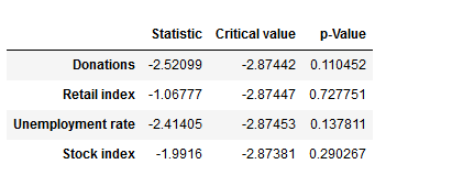
 Particularly in uncertain times like these, organizations strive to predict the future in the best possible way. Previously we have already explored multiple times how to forecast future income using the past income trajectory, for instance in these blog posts. We now want to go a step further and investigate the relationship between fundraising income and the general economic climate, exploring whether or not it is possible to infer extra information from and improve income forecasting tools by using economic indicators.IntroductionMore specifically, we will look at correlations between the amount of sporadic donations to a charitable non-profit organization from the period of 2000 to 2019 and three economic data sets from the country the NPO is based in: the national unemployment rate, the national stock market index and an index of economic activity in retail, authored by the national bureau of statistics. We chose these data sets for their ability to paint a picture of the general economic climate, their relatively easy accessibility down to the monthly level and the fact that to the extent that they exhibit seasonality, they do so in the same yearly rhythm as the amount of sporadic donations, simplifying the statistical analyses. The statistical analyses and models employed in this blog post were all implemented in Python, taking heavy use of the statsmodels library. The main mathematical tool used for the analyses is a time series, which is a set of data points collected over a discrete, ordered time. We have already looked at time series in detail in a past entry on this blog. An important property of time series is that of stationarity, which we discussed here. As in that post, we use the Dickey-Fuller test to investigate whether or not our time series are stationary, which can be done in python like this: Dickey-Fuller test
We have defined a function that returns a dataframe with the test statistic, the critical value at a confidence level of 5% and the p-value for the Dickey-Fuller-Test for each time series. The p-values of the test results are above a significance level of 0.05, leading us to keep the null hypothesis of the time series being non-stationary. In cases like these, differencing the time series – this means subtracting the previous value from the current – can help in making the season stationary. However, due to our time series exhibiting strong yearly trends, in our case it makes sense also to take the time series’ seasonal differences, subtracting the values from the year before. Granger causalityHaving prepared our time series, we can look at a first test of interdependencies. Using a version of Pearson’s Chi-Squared test, we examine the (made stationary) series’ Granger causality, which tells us whether data from one series can help in forecasting the future trajectory of another series. The test is applied pairwise on two different time series, with the null hypothesis being that the second time series does not Granger cause the first. The following function returns a data frame that shows the p-values of the tests investigating whether the column variable granger causes the row variable. Especially the first row – indicating (no) Granger causality between the economic data sets on the one hand and the amount of sporadic donations on the other – is interesting to us. At a significance level of 0.05, we keep the null hypothesis of no Granger causality between the economic indicators and the sporadic donations for all three time series. Granger causality
CointegrationA second useful quality to look at is cointegration. We consider a set of time series cointegrated if there exists a linear combination of the time series that is stationary. Cointegrated time series share a common, long-term equilibrium and we can use them to predict each other’s future trajectory using a process called Vector autoregression (VAR). A common test for cointegration is the Johansen cointegration test. In the following, we define a function that returns a dataframe with the test statistic and the critical values of the Johansen test, leading to these results: Johansen cointegration test
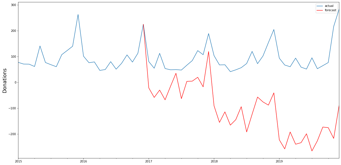
The test statistic is below the critical value for all four of our time series, meaning that we have to keep the null hypothesis of no cointegration and cannot assume the time series to be cointegrated. We can thus not assume that there is an underlying equilibrium between the four time series, and the test results do not support the hypothesis that we can use the time series to forecast each other’s future trajectory. Vector autoregression (VAR) Had the test results been different and had we been able to reject our null hypothesis, we could have attempted to construct a VAR-model. If we ignore our test results for a moment and do so anyway, we can immediately see that the model falls catastrophically short. The black line in the below graphs show the actual time series of sporadic donations. Having used data until 2016 as our training set, we constructed with the Python library statsmodels a VAR-model that we can use to forecast the sporadic donations from 2017 to 2019 – the red line in the graph – using the actual data for these years for evaluation. As we can see, the model is not able to forecast the amount of sporadic donations very well, capturing the seasonality, but failing to accurately predict the trend and overall trajectory. Vector autoregression
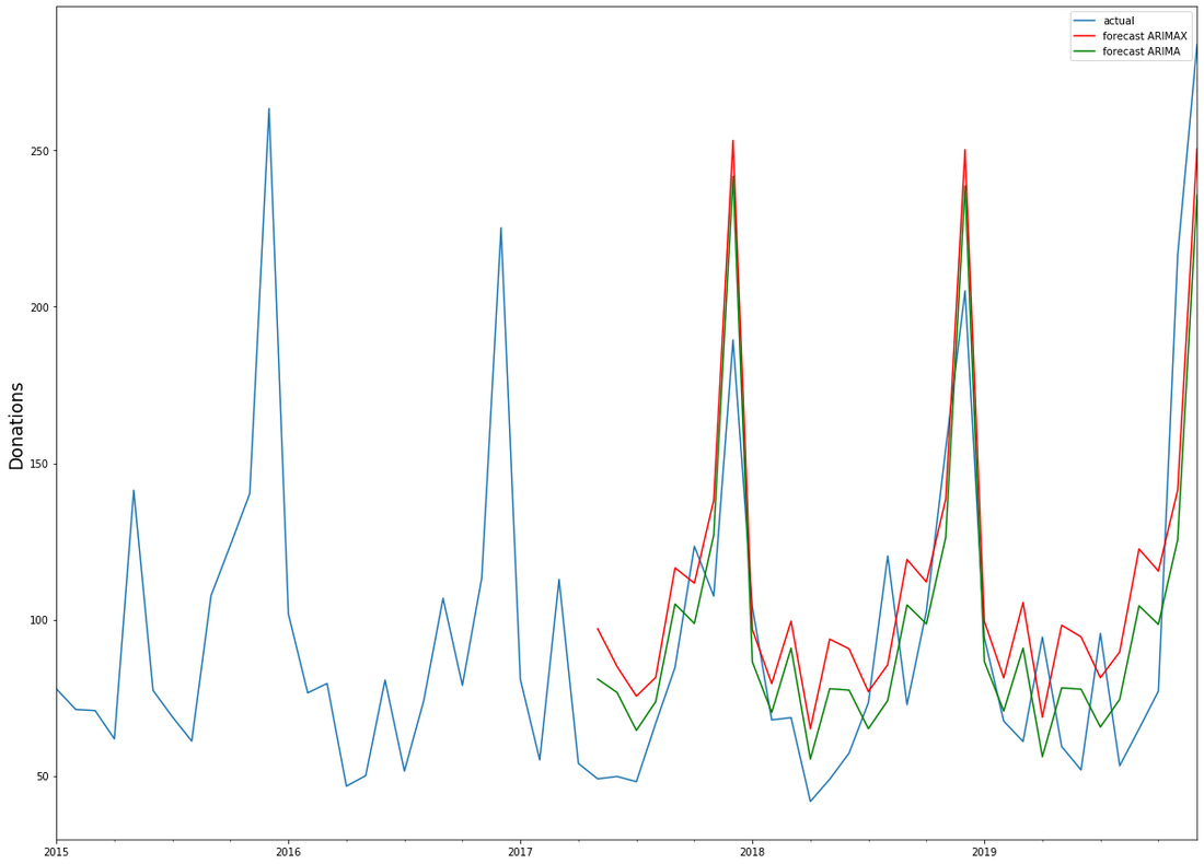
ARIMA and ARIMAXUsing a different model does not yield any much better results. We attempted to construct an ARIMAX-model, a generalisation of the ARIMA-model, which we have used previously in this blog, that also takes into account data from external variables – in our case, the economic time series. ARIMA models are composed of three parts: AR for autoregression, indicating a regression on the time series’ past values, I for integration, signifying differencing terms in the case of a non-stationary time series, and MA for the moving-average-model, a regression on past values white noise terms. ARIMAX takes all three of those terms and adds data from external variables – a different time series – to better forecast the time series at hand. Both ARIMA and ARIMAX are implemented in python as part of the statsmodels library, while the pmdarima library comes with an autoarima function modelled on R’s autoarima function, allowing for a quick search through the possible parameters of the ARIMA(X) model. We have used all four time series to construct an ARIMAX-model, using the economic data to help forecast the amount of sporadic donations. Again we used the data until 2016 as our training set, with the data from 2017 to 2020 as a test set to evaluate results. We have also used a standard ARIMA-model to construct a forecast for sporadic donations only on the time series’ historical data. Interestingly, the models’ projected forecasts did not differ much from each other: ARIMAX
It seems thus that the economic data we have provided – the unemployment rate, the stock index and a retail index – did not add much extra information to better forecast the amount of sporadic donations. Upon closer inspection the ARIMA-model, relying solely on historical data from the time series itself, even performed slightly better. In light of the previous test results – the lack of Granger causality and cointegration – this points to the fact that those economic indicators have little measurable effect on the development of sporadic donations, and thus cannot be used to improve forecasting models for the amount of sporadic donations in the future. However, we believe that the approach of using time series analysis for fundraising income predictions hand in hand with open (economic) data deserves further focus as other base data, time frames, data sources etc. might lead to different results!
1 Comment
|
Categories
All
Archive
June 2024
|


